Investigating the Average Change of A Rate

There are multiple mathematical solutions for real-life situations, but the Average Rate of Change stands out, because of its versatility. Let’s take a closer look at the fundamentals of this instrument and review the ways of its utilization.

Definition

First of all, the Rate of Changes provides the user with a great portion of knowledge about the relation between one quantity and another: the working principles are gathered around measuring the speed of the observed quantity’s changes.

However, there are two separate types of this value: average and instantaneous. Both of them evaluates different aspects of the quantity:

1. Instantaneous Rate of Change investigates a single point of time.
2. Average, on the over hand, observes the overall, total changes throughout the whole time period.

There is another crucial part in such calculations and that is the limits which prior goal is to make the shift between an Instantaneous Rate of change to an Average greatly smoother. Such limitations make these measurements happen, because it would be simply impossible to define the value without a clear borderline.

Based on principles of work, this rate becomes, especially, valuable in cases of observing motion, growth tendencies and many other processes which occur through a continuous amount of time.

Measuring

To start with, there is the Average Rate of Change formula:

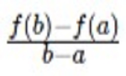
Let’s analyse the prior features of this equation.

The analytical depth of these expressions lays in the relation between two functions which helps to discover the overall increase or decrease of the function throughout the measured time frame.

It is crucial to know that the difference between b and a can’t equal zero, because the equation won’t have any meaning: it’s down to the fact that the division by 0 is impossible. Consequently, both a and b must have different values due to this rule. Moreover, these function values must be defined to make the expression have any sense in the end.

Instance

Let’s review a hypothetical instance of the Average Rate of Change where the following variables are 3 and 6. The function formula is going to be: f(x) = x^2. Now, the solving and measuring step-by-step:

1. Definition of the existing function and both its endpoints: f(x) = x^2. The endpoints are identified as: a = 3 & b = 6.
2. The next step is to calculate both f with such values: f(3) = 3^2 = 9 & f(6) = 6^2 = 36.
3. Integrating the resulting numbers into the existing formula of the Average Rate of Change: (f(6) – f(3)) / (6 – 3) = (36 – 9) / 3
4. Simplify the resulting expression: 27 / 3 = 9.

As it stands from the result, the Average Rate of Change of the function from 3 to 6 is 9. Let’s review it in a more detailed way: the identified function “f(x) = x^2 has an increase by 9 during every single increase in x throughout the existing time interval.

Comparison of the Average and Instantaneous

However, the features that the Average Rate of Changes provides the observer with wouldn’t be enough to define what occurs at the specific single point. In that case, the Instantaneous Rate is quite useful due to the fact that its prior goal is to determine the speed of the function changes in the exact single moment.

The existing limits help to overcome the gap between the Average and Instantaneous Rates. The Instantaneous Rate can be discovered by making the existing interval points infinitely close to one another. The values which are revealed are the derivatives.

Instantaneous Change Instance

Let’s review a hypothetical instance of the Instantaneous Rate which also contains the same formula: f(x) = x^2 where the x = 4 while utilizing the f’(x) which is the limit definition of the derivative. Now, the calculations step-by-step:

1. Determine and state the limit definition: f’(x) = lim (from h to 0)(f(x + h) – f(x)) / h.
2. Use the existing value of x and integrate it in the formula: f’(4) = lim (from h to 0)((4 + h)^2 – 4^2) / 2.
3. Execute the calculations and make the equation more simple: (4 + h)^2 = 16 + 8h + h^2.

In that case, the existing resultings will look like this: (16 + 8h + h^2 – 16) / h or (8h + h^2) / 2.

1. Make the dividing by h: (8h +h^2) / h = 8 + h
2. Define and include the limit as h reaches zero: lim (h to zero)(8 + h) = 8.

In that case, if x = 4 within the f(x) = x^2, the instantaneous Rate of Change will be equal to 8 which is the speed of the function change at the exact point of x = 4.

Ways to utilize

There are multiple ways to utilize this mathematical tool and here are several of them:

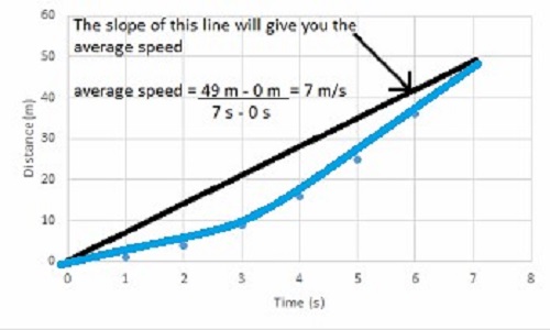
• To measure the average speed of a moving vehicle. Physics often requires such measurements, especially in the case of engineering.

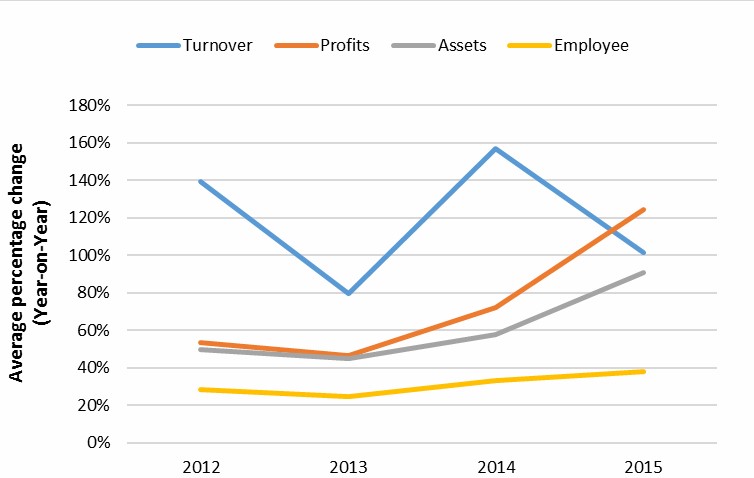
• Identifying the overall annual increase rate of a company or business. This is a crucial date which provides the investor with more sophisticated knowledge that will help to make a more qualified decision.

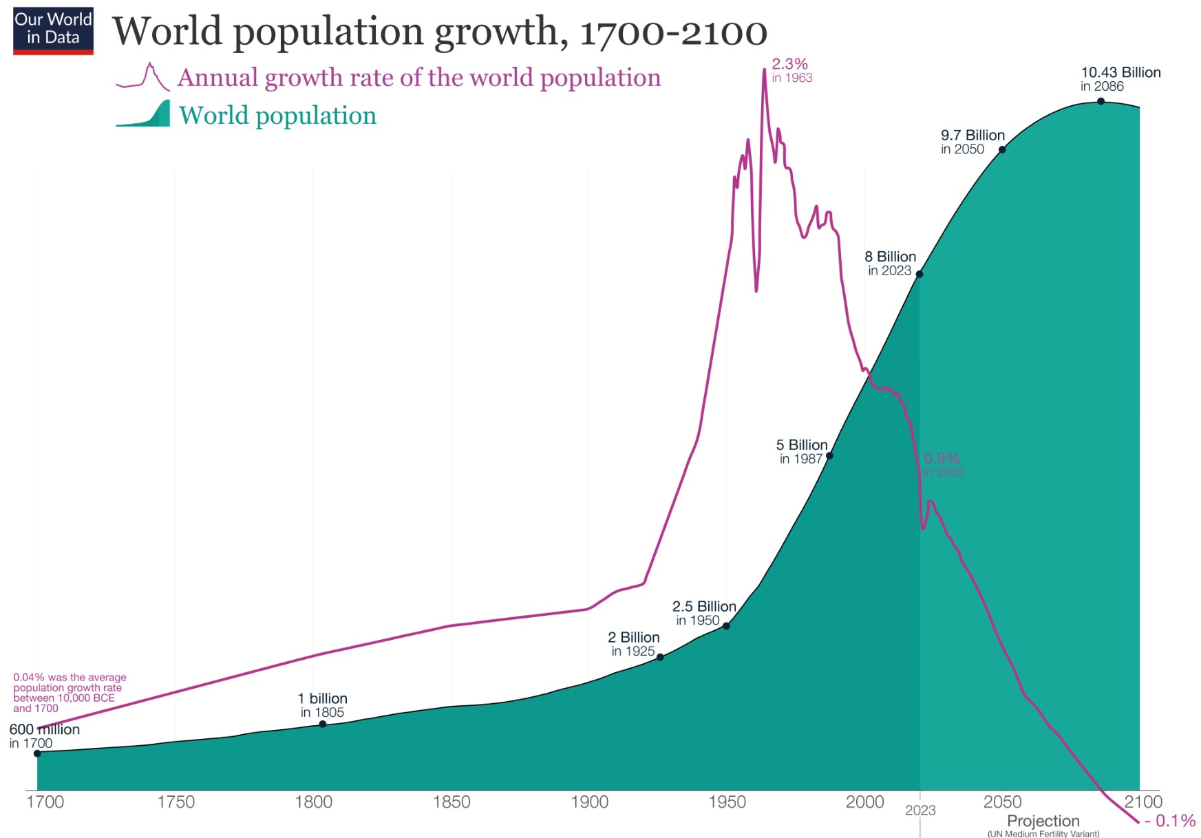
• Making the predictions of the population increase.

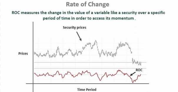
• Calculating the stock’s average rate of change. Like investigating a company, it is a crucial way to increase the potential of gaining profit: such rates will reveal the asset’s behaviour over a period of time. The knowledge base of the trading strategy is fulfilling with the Average Rate of Change.

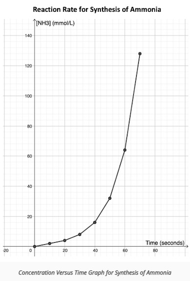
• Identifying the overall speed of chemical reactions. Due to the fundamental principles of science, it is also a crucial tool in the hands of the chemistry scientists. The collected data add the explanations of the chemical reaction’s kinetics.

However, there are more ways to integrate this mathematical tool to the variety of real-life situations. It also means that this is a crucial and versatile instrument.

FAQ

What is the Average Change of Rate?

The Average Rate of Changes provides the user with a great portion of knowledge about the relation between one quantity and another: the working principles are gathered around measuring the overall speed of the observed quantity’s changes during a continuous amount of time.

What is the Formula of the Average Change of Rate?

There is a formula of Average Change of Rate:

How to utilize the Average Change of Rate?

There are a variety of ways to use it. The user can measure the Average Rates of: moving vehicle speed, company’s annual growth, the population growth, stock’s changes and e.t.c. It is one of the most versatile tools to use in the calculations of the overall variables.